Sign up for the ITPro Today newsletter
Stay on top of the IT universe with commentary, news analysis, how-to's, and tips delivered to your inbox daily.
Expanding your repertoire of entity relationships beyond the usual parent-child hierarchy structure could pay off big.

Multifaceted entity relationships: graphs and maps
Some of the most common, and often flawed, models in relational database management systems (RDBMSs) are dependent on the structures (such as trees, graphs, and maps) necessary for storing entity-to-entity relationships. You need self-referencing tables and their respective parsing mechanisms to model generations and genealogies (trees), organization charts (graphs), and geographies (maps). Using a geographic database as an example, this article explores trees, graphs, and maps and looks at how to extract the data from these structures.
Database modelers are often guilty of taking a few shortcuts when performing the onerous task of saving geographical taxonomies in a database. We take these shortcuts and fulfill the requirements, although we know that the requirements haven't taken into account the inevitable scope expansion that is typical of any growing organization. Almost every database in production must have the facilities to store hierarchical data. This article's example focuses on geographic data, but hierarchical data is prevalent in many of today's models. The example database requirements specify that the database must support state and city information. The implementation of only two generations of data appears simple enough—a one-to-many (1:M) relationship will suffice. You know that eventually you'll have to redesign this database relationship; when the company starts selling its product outside the United States, the new requirement will specify that the database needs more than a region-subregion relationship. If you're fortunate, you'll only need to add a third table for country information. If not, you'll need to totally redesign this database model, which takes time and money.
Further investigation of the data in geographic information systems (GIS) map software reveals that countries have complex and disparate organization structures. Some countries are organized by state, others by region or province. Using small areas of the United States and South Africa as examples, you'll find the hierarchies that Figure 1 shows. The disparity in structure between the two countries in Figure 1 shows that you can't model generic organization charts by using a simple 1:M relationship because you can't predict the depth of the hierarchy. In this example, you can see that countries don't abide by an organizational standard. The United States is segmented into states and districts, both of which contain cities. Other countries might be divided into provinces or regions, or perhaps not be subdivided at all. Other hierarchies such as genealogies and corporate organization charts have the same problem. When confronted with disparate organizational structures, many developers opt to use self-referencing tables. One column in every self-referencing table has a foreign-key relationship with another column in the same table. Listing 1 creates a table called Entity, in which entIDEntityParent is a self-referencing column; you can use this table to store the geographic data for our example.
Why did we prefix every column with the characters "ent"? By assigning each table a unique three-character prefix and prefixing every column with the table prefix, you eliminate the need to alias all your joins when you begin creating dynamically generated SQL statements. (You might use dynamically generated SQL to search for a certain piece of data based on user-specified input. Constructing the SQL dynamically lets you omit superfluous joins and thereby increase query performance.) Making all the column names unique could save you hundreds of hours of creating these customized SQL generators. Also, naming the table Entity and not GeographicLocation or something similar provides for maximum reuse because naming the table Entity lets you use this table to store any kind of entity. You can use this table as a template for a domain value table in which you can store any kind of lookup data. (Of course, you might need to add a few more columns as you internationalize—e.g., for language IDs.)
The first column in the Entity table is entIDEntity; this column is a unique identifier that acts as the primary key. Note that we didn't use an integer data type for the IDENTITY column. We recommend that you use the uniqueidentifier data type (new in SQL Server 7.0), provided you take into consideration the 16 bytes of space a globally unique ID (GUID) requires for storage, indexes, and joins. SQL Server developers tend to avoid GUIDs, using integers instead for portability reasons. But using GUIDs will yield benefits if you decide to configure replication. Regarding the use of unique identifiers in replication, SQL Server Books Online (BOL) says: "If you are using merge replication, or if you are using snapshot replication or transactional replication with queued updating and the table that is being replicated does not have a uniqueidentifier column, SQL Server 2000 will add one when you create a publication."
The table's second column, entName, is the field you use to store the country, city, or region name—the friendly name that you present to your users. You can use the third column, entType, to identify the type of entity—e.g., country, state, or city. Finally, the entIDEntityParent column identifies each entity's immediate parent. This self-referencing column works well for the trees that Figure 1 shows. For every entity, you can store the uniqueidentifier of its parent in this column.
What happens when your database needs to support an organizational structure in which entities can have multiple parents? The table from Listing 1 won't support multiple parents because the relationship is stored with the entity definition. Because you can have only one instance of an entity definition, you're inherently limited to only one relationship for the entity. In a typical hierarchy model or tree, the table in Listing 1 would be fully functional because nodes in a tree have only one parent. (For more information about hierarchy models, see Itzik Ben-Gan, "Maintaining Hierarchies," July 2000.) However, with multiple parents, this structure is no longer a tree; it's a graph, typical of what you might find in genealogy trees or geographical structures. Why would you need to support multiple parents in a GIS environment? Let's say you want to provide an Internet city-search portal where users can search for cities by state, by county, or by area code. But some cities have multiple parents: A user searching by area code would find San Francisco as a city in two area codes, 650 and 415, as Figure 2 shows. So, San Francisco has more than one parent. This example might seem trivial; however, the concept of an entity having more than one parent is crucial in many other situations. For example, in genealogies, humans have two parents—sometimes more if you include stepparents.
Entities that have multiple parents can be problematic for the geographic database model because the model provides for only one column in which to store the entity's parent. Up to this point, you were dealing with entities that have only one parent (a tree), but now you have entities with multiple parents (a graph). Fortunately, a solution is close at hand: Just remove the self-referencing column from the entity table. Listing 2 removes that column and creates a new table called EntityRelationship. Removing the self-referencing column abstracts each entity from its parent-child relationship, thereby letting one entity be involved in more than one parent-child relationship. In other words, some hierarchies involve many-to-many (M:N) relationships, and this EntityRelationship table is an intersection table that resolves the M:N relationship.
Let's consider the alternatives to creating this intersection table. Merely duplicating the entity with a new ID would probably work when the entity has no related records. However, if you decided to duplicate the entity, you would have to manually maintain this duplication of information because the duplication violates the rules of normalization. So, when is denormalization appropriate? The only reason to denormalize data structures is to increase performance. The process of denormalizing can speed up data access but requires increased programming to maintain the denormalized data. An example of denormalizing is storing account balance information along with a customer record. Although you could compute the balance by calculating all transactions, doing so is time-consuming, so DBAs often save the account balance with the customer record. This denormalization results in increased performance—and in more programming. (See Michelle A. Poolet, Solutions by Design, "Responsible Denormalization," October 2000, for denormalization suggestions.) But in a geographic database, and for that matter most databases irrespective of industry, duplicating the entity isn't feasible because of the potentially large amount of information associated with each entity record.
Using our new model, you define an entity in the Entity table, then you define all the entity's relationships in the EntityRelationship table. Consequently, an entity can now have multiple parents. However, the column combination of eteIDEntityChild and eteIDEntityParent becomes the primary key, thus enforcing the restriction that any entity can have only one occurrence of the same parent.
Just when you think you're ready to deploy your database, you receive a new requirement—to create sibling relationships among entities. Your company wants the Internet city-search portal to track climatic similarities among cities so that when a user searches for a city, the program also shows other cities that have similar climates. In Figure 3, the climatic and scenic relationship between Cape Town and San Francisco is not a parent-child relationship like the Figure 1 country scenario. Thus, the existing database structure no longer works because the EntityRelationship table can't differentiate between a parent-child relationship and a sibling-sibling relationship. To solve this problem, you can use the code in Listing 3, page 58, to modify the EntityRelationship table.
The code renames the fields from eteIDEntityChild and eteIDEntityParent to eteIDEntity1 and eteIDEntity2. The new field called eteRelationship abstracts a parent-child relationship to a generic relationship; now the database design can support many different types of relationships. Because eteIDEntity1 and eteIDEntity2 can have numerous distinct relationships with one another, we added the eteRelationship field to the primary key, as Figure 4 shows, so that you can relate two entities to each other in more than one way. For example, you can relate Cape Town to San Francisco by climate, by landscape, and perhaps even by size. When innumerable types of relationships exist between entities, you have multifaceted relationships. Although these relationships can be difficult to maintain, it is precisely these relationships, deciphered from sophisticated data-mining processes, that let Internet sites upsell and cross-sell. Upselling a product is easy—you just define an Upsell relationship between a particular product and the products that are more expensive versions of it. Cross-selling is just as easy—you define a Cross-Sell relationship between the product and its associated products. Within the Cross-Sell relationship, you could even define Dependency or Accessory relationships (remember, batteries and accessories are hardly ever included).
Several years ago, marketers found a relationship between sales of beer and sales of diapers. The two items had similar purchase times, which at first seemed coincidental. However, further examination revealed that parents would pick up diapers after work and would take the opportunity to grab some beer (or vice versa). So the marketers moved premium beer next to the diapers—and in so doing, they increased premium beer sales.
The future of data mining lies in deriving these relationships and exposing them to smart applications, which can use the relationships to increase sales. Anyone who's visited Amazon.com has probably experienced cross-selling. Personalization, an area based on exposing related data, enables such cross-selling. (For more details about data mining, see Barry de Ville, "Data Mining in SQL Server 2000," January 2001.) Now with the data model we've established, you can capture these relationships by inserting the appropriate relationship records into the EntityRelationship table. Geographic regions, for example, can have many relationships with each other, such as bordering countries/states/regions, demographically similar, or populationally similar.
Let's refer back to the EntityRelationship table now that you see how to identify different types of relationships. You might be concerned about the data type of the column that stores the relationship indicator. In a production system, this column should be a uniqueidentifier data type to increase the performance in accessing this table. But it's OK to cheat a little, especially for readability purposes while you're getting things up and running. For performance reasons, you just need to change this data type when you go into production.
Many SQL Server developers have difficulty extracting data from a hierarchical structure. Your next assignment is to provide the appropriate SQL statements to give Internet users efficient access to the tables you created to house entity relationships. For the example data, let's model a little of Earth's geographical map; Figure 5 contains some sample data. Data that is derived from tables containing hierarchical data is often presented in a Web-based tree control. Have you ever noticed how some Web pages seem to take an inordinately long time to expand a tree control? During the delay between every click of the + sign, these pages are actually performing a round-trip to the server for every node in the tree. They are issuing database requests to the server to retrieve the children of the node you just clicked.
Performing numerous round-trips to a database is an extremely inefficient means of interacting with both the database and the user, for several reasons. Mainly, a Web page is largely ineffective as a means of interacting with a user if the user must wait several seconds between clicks. Internet users generally will wait a few extra seconds up front if their subsequent successive requests are instantaneous. Also, every round-trip to the database has associated overhead, including database connection time, SQL parsing, and SQL execution-plan generation.
A preferable means of implementing the tree control is to download the entire result hierarchy at the first request, then use Dynamic HTML (DHTML) to expand the tree. The only drawback of such a design is that you might be transferring an enormous data set. If your tables contain tens of thousands of records (e.g., if you were trying to present a list of cities by country), you might first filter the resultset by asking the user to specify a subset of the data (perhaps through a combo box selection) before issuing the SQL statement to download the cities.
But before you can code the HTML to present your data, you need to write the SQL statements that will extract data and send it to the client. Using a tree control, the client will ultimately render the resultset data on the screen. The SQL statements that generate the resultset will be part of a stored procedure, which begins at a specified starting point and returns a set of records containing all related entities.
Before diving into a subterranean exploration of the SQL composing this stored procedure, which Listing 4 shows, let's take a hundred-foot view. The goal of this stored procedure is to find all entities that are related to the starting point. Using our previous example, your starting point might be San Francisco, in which case the stored procedure would return all entities that have any relationship, direct or indirect, with that city. This example uses the Planet Earth record as a starting point for retrieving all related records, which should be all the records in the table. The records returned will contain information about what entity each is related to, how many levels separate them from the starting point, and so on. Using the resultset, HTML programmers can render the entire tree control without the need for successive round-trip database requests, because the resultset contains the relationships between entities, rather than the entities themselves.
The procedure starts by creating a temporary table called #Map, which it will use as a symbolic data stack. (The stack is symbolic because SQL Server has no inherent stack capabilities, but you can simulate a stack by using a field called Processed in the #Map table.) The procedure pushes records onto the stack, then pops them off the stack. If the Processed field's value is set to 0, the record is considered to be on the stack; if the field's value is 1, the record is considered to have been popped off the stack. After creating the #Map table, the code proceeds by pushing the first record onto the stack; this record is the starting point from which the code will begin to look for related records. The procedure then enters a looping structure, which pops the top record from the stack. The procedure uses this record to find related records, which the procedure subsequently pushes onto the stack. When the stack is empty (i.e., all records have the Processed field set to 1), the procedure returns the records it found and stored in the #Map table, and you're done.
Note that this stored procedure will return all entities related in any way to the starting point. If you want only the entities of a certain relationship type, you need to modify the stored procedure. For example, if Person A is related to Person B by a "blood relationship" and Person B is related to Person C by a "friend relationship," then with Person A as a starting point, the procedure will return all three because A is related to B and B is related to C, making C related to A. To find only the persons related by blood to Person A, you need to modify this stored procedure by specifying the relationship type in the WHERE clause. Now let's go through the SQL code in Listing 4 in more detail.
Callout A in Listing 4 defines the stored procedure name as ap_Map_Traversal. The prefix "ap" signifies that the procedure is an application procedure and not a system procedure. This nomenclature helps when you want to easily differentiate Microsoft-supplied procedures from those you need to run your application. The procedure takes one parameter, @startPoint, which is an entity identifier; the procedure will begin looking for related entities from this origin point. If the parameter value is null, Callout B initializes the starting point to a default starting point. You need to adjust SET NOCOUNT ON to reflect your default starting point.
Callout C declares an integer variable, @level; the procedure will use this variable as a counter that reflects the number of levels that separate an entity from the starting point. Callout D creates the #Map temporary table. The #Map table has six columns:
Item—contains the entity's unique identifier
ItemName—contains a descriptor for the entity defined in the Item column
RelatedToItem—contains an entity's unique identifer, to which the Item column is related by the relationship specified in the Relationship column
Relationship—contains the relationship type by which RelatedToItem and Item are related
Generation—contains an integer value that specifies the number of levels by which the item is separated from @startPoint, which has a generational value of 1
Processed—contains a value of 0 or 1, specifying whether the point (as defined by the Item column) is awaiting processing or has completed processing
Callout E inserts the root node into the temporary table #Map. Callout F initializes the @level variable value to 1. Callout G comprises the looping structure, which will loop as long as the @level variable is greater than 0. In effect, the variable acts as an altimeter—it measures how far from the starting point each entity is. As the result items' generations get further from the starting point, this variable's value increases, and as they get closer to the starting point, the variable's value decreases. When the variable's value is 1, the procedure is back at the starting point; when the value reaches 0, the procedure has processed all records related to the starting point, and the loop construct is finished.
Now we enter the loop. Callout H provides the SELECT statement to check for the existence of records that are awaiting processing. If no records are found, the @level variable is decremented by one (Callout I). If records exist, execution continues with Callout J, at which point the code extracts only the top record's Item value and sets the Processed column value to 1 (popping the record off the stack). The INSERT statement in Callout K adds into the #Map table all records the Item is related to and sets the Processed column to 0, pushing the records onto the stack. Note that the procedure sets the Generation to the current generation's value plus 1 because these records are separated from the starting point by a generation, so for the first time through the loop, the generation would be incremented to the value 2.
You can determine whether records were inserted into #Map by querying the global variable @@rowcount, which returns the number of records affected by the last statement executed. If this value is greater than 0, records were inserted, so you need to increment the @level variable so that the next iteration through the WHILE loop will process the subsequent generation. The execution follows a Depth First Search (a means of traversing data in which you exhaust depth before breadth) approach to processing. Processing will continue in this way until the procedure has exhausted all records in the #Map table, at which point the @level variable's value becomes 0. This value causes the loop to terminate and the procedure returns the contents of the #Map table through Callout M. Figure 6 shows the final output of running this procedure.
The T-SQL code in Listing 4 works well with data in which no circular relationships exist. If Person A is related to Person B by a "blood relationship" and Person B is related to Person C by a "friend relationship" and C is related directly to A, you have a circular loop in which A is related to C, who is related to A. Maps are structures that contain these circular loops; maps are nonlinear, nonhierarchical points connected by bidirectional lines—the very essence of multifaceted relationships. So although the stored procedure code in Listing 4 works when only one path exists between two points, it fails when it encounters a loop formation such as a multifaceted relationship. The code will enter into an infinite loop as it tries to process nodes that have children that are in their own ancestry. For example, suppose you add to the EntityRelationship table the two records that Figure 7 shows. The records establish a relationship between North America and Canada as parent and child and between the United States and Canada as trading countries. After you insert these records, rerun the stored procedure. The stored procedure never returns because it has entered an infinite loop; if you let the stored procedure run indefinitely, it will raise an error when the #Map table has exhausted database capacity.
The solution to this infinite loop asserts practicality over elegance. You need an indicator to tell the procedure that it has encountered a loop—in other words, a point that has already been processed. In some implementations, the indicator is part of the data itself. For example, some implementations contain special columns that indicate a loop if the value is set to 1; however, such an implementation is inadvisable because it renders the entire solution data-sensitive. A data-sensitive solution requires that the person who writes the code to traverse the map have complete control over the data generation. Getting this control is unlikely, especially when you're trying to integrate with a third-party data provider. We encountered this type of situation when working on a project in which a law-enforcement agency acquired $10 million worth of proprietary data from the local electric utility company. The utility company wasn't about to change millions of records—so we needed to write a stored procedure that would not go in circles ad infinitum.
The ideal solution is to have the procedure keep a list of all points processed, then before processing any point, verify that it hasn't already encountered the point. If the procedure has processed the point, it can simply skip that point. Because the #Map table is a list of points that are either pending processing (Processed column = 0) or already processed (Processed column = 1), the solution is simple. Inserting the following T-SQL clause into Listing 4 at Callout L will prevent the insertion of entities that already exist in the #Map table.
AND eteIDEntity2 NOT IN (SELECT relatedToItem FROM #Map)Now if you rerun the stored procedure, you will find that it no longer encounters an infinite loop, but returns the resultset correctly. Congratulations! You are now in a position to effectively manipulate complex data involving multifaceted relationships. Your database model can now support complex organization charts, genealogies, geographical data, and any other relationships by which two entities can be related in more than one way. Now be sure to model those simple country, state, and city relationships the right way—no shortcuts!
You May Also Like


.jpg?width=700&auto=webp&quality=80&disable=upscale)